Showing posts with label Math. Show all posts

Wednesday, January 4, 2017

D&D Stat Roles

If you have played any incarnation of D&D, you are no doubt familiar with the ritual of generating the vital statistics defining your character:

  • take four D6s, roll them, throw away the lowest one, and sum up the remaining three
  • repeat the above five more times, giving six numbers
  • assign these numbers among strength, fortitude, dexterity, intelligence, wisdom, and charisma

In this post, we will examine the question: what are the odds of a given stat number being rolled?

The answer is trivial to produce for a competent programmer, and is as follows:

Stat rollOdds
3 1 in 1296
4 4 in 1296
5 10 in 1296
6 21 in 1296
7 38 in 1296
8 62 in 1296
9 91 in 1296
10122 in 1296
11148 in 1296
12167 in 1296
13172 in 1296
14160 in 1296
15131 in 1296
16 94 in 1296
17 54 in 1296
18 21 in 1296

This isn't a very satisfying answer, though. Why is the table the shape that it is? Compare the table above to the following table, which is the odds of 3D6 summing to a given number, with no throwing away of any dice:

Stat rollOdds
3 6 in 1296
4 18 in 1296
5 36 in 1296
6 60 in 1296
7 90 in 1296
8126 in 1296
9150 in 1296
10162 in 1296
11162 in 1296
12150 in 1296
13126 in 1296
14 90 in 1296
15 60 in 1296
16 36 in 1296
17 18 in 1296
18 6 in 1296

The distribution for 4D6 with a dropped die is more complex because the final sum depends critically on which die is the lowest (and thus thrown away), but the odds that a given die is the lowest is dependent on the value rolled on the other three dice.

To be specific: say you rolled the first die, and it came up a 1. In this case, you would know that this was the lowest roll, and could consider the odds of the final sum assuming that that die was thrown away. If the first die rolled a 6, you would know that this was NOT the lowest roll (at the worst it was tied), and could keep it, and odds of the final sum could be the odds of 3D6 were rolled, and one was thrown away, and you added six to that total. If, however, the first die was any other number, you really don't know very much. You have to roll the others to see.

To make headway on our problem, we need to separate these dependencies into a set of disjoint, indepenent possibilities. We do so by observing two facts:

  • For any 4D6 roll, exactly one is true: the first die is lowest, the second die is lowest, the third die is lowest, or the fourth die is lowest
  • For any 4D6 roll, exactly one is true: the lowest die is a 1, the lowest die is a 2, the lowest die is a 3, …, or the lowest die is a 6

One more fact is required, to handle the case where the lowest number is rolled more than once (for example the roll {3,1,1,6}). In such a case, the lowest die is the first one with the given lowest roll.

Convince yourself that every 4D6 roll will fall into one of these 24 buckets:

Lowest rollLowest die
1st2nd3rd4th
1
2
3
4
5
6

Let us begin to fill in the table:

  • What are the odds that the lowest roll is a 6?
    • Clearly, this will only happen if all four dice roll 6, and this can only occur once.
  • What are the odds that the lowest roll is a 5?
    • This occurs if all four dice roll 5 or 6, which can occur 2^4 = 16 times. However, we must subtract one, since we have double-counted the case where all four dice roll 6.
  • What are the odds that the lowest roll is a 4?
    • By a similar argument, this will be 3^4 - 2^4 = 65
We continue this line of reasoning, and are able to conclude that:
Lowest rollLowest dieRow sum
1st2nd3rd4th
1671
2369
3175
465
515
61

We don't yet know what is in each bucket, but we can sum the rows of the buckets.

Now, consider the case where the lowest roll is a 1:

  • What are the odds that it is the first die that rolls 1?
    • To do this, the first die must roll 1, and then the other three dice rolls can be anything. They thus fit the pattern [1][*][*][*] (where * denotes 'any'). This has 1*6*6*6=216 occurrences.
  • What are the odds that it is the second die that rolls 1?
    • Recall the rule that the lowest die is the first with a given value. For the second die to be the lowest, and have rolled 1, the first die cannot roll 1. We thus have the pattern [2+][1][*][*], which has 5*1*6*6=180 occurrences.
  • What are the odds that it is the third die that rolls 1?
    • By a similar argument, rolls of this type fit the pattern [2+][2+][1][*], which has 5*5*1*6=150 occurrences.
  • What are the odds that it is the fourth die that rolls 1?
    • By a similar argument, rolls of this type fit the pattern [2+][2+][2+][1], which has 5*5*5*1=125 occurrences.

As a check of our reasoning, observe that 216+180+150+125=671. We can thus fill in the table as follows:

Lowest rollLowest dieRow sum
1st2nd3rd4th
1 [1][*][*][*] (216) [2+][1][*][*] (180) [2+][2+][1][*] (150)[2+][2+][2+][1] (125)671
2[2][2+][2+][2+] (125)[3+][2][2+][2+] (100)[3+][3+][2][2+] (80)[3+][3+][3+][2] (64)369
3[3][3+][3+][3+] (64)[4+][3][3+][3+] (48)[4+][4+][3][3+] (36)[4+][4+][4+][3] (27)175
4[4][4+][4+][4+] (27)[5+][4][4+][4+] (18)[5+][5+][4][4+] (12)[5+][5+][5+][4] (8) 65
5[5][5+][5+][5+] (8) [6][5][5+][5+] (4) [6][6][5][5+] (2) [6][6][6][5] (1) 15
6 [6][6][6][6] (1) 1

Note that the tiebreaking rule results in three of the buckets being empty.

"So what?" I hear you now ask. "You have taken one number and split it into the sum of twenty-one different numbers. How does this help?" I respond by first noting that the identity we have discovered is not at all obvious, and can be admired in its own right:

6*6*6 + 6*6*5 + 6*5*5 + 5*5*5 + 5*5*5 + 5*5*4 + 5*4*4 + 4*4*4 + 4*4*4 + 4*4*3 + 4*3*3 + 3*3*3 + 3*3*3 + 3*3*2 + 3*2*2 + 2*2*2 + 2*2*2 + 2*2*1 + 2*1*1 + 1*1*1 + 1*1*1 = 6*6*6*6
        6*6*5 + 6*5*5 + 5*5*5 + 5*5*5 + 5*5*4 + 5*4*4 + 4*4*4 + 4*4*4 + 4*4*3 + 4*3*3 + 3*3*3 + 3*3*3 + 3*3*2 + 3*2*2 + 2*2*2 + 2*2*2 + 2*2*1 + 2*1*1 + 1*1*1 + 1*1*1 = 6*6*6*5
                6*5*5 + 5*5*5 + 5*5*5 + 5*5*4 + 5*4*4 + 4*4*4 + 4*4*4 + 4*4*3 + 4*3*3 + 3*3*3 + 3*3*3 + 3*3*2 + 3*2*2 + 2*2*2 + 2*2*2 + 2*2*1 + 2*1*1 + 1*1*1 + 1*1*1 = 6*6*5*5
                        5*5*5 + 5*5*5 + 5*5*4 + 5*4*4 + 4*4*4 + 4*4*4 + 4*4*3 + 4*3*3 + 3*3*3 + 3*3*3 + 3*3*2 + 3*2*2 + 2*2*2 + 2*2*2 + 2*2*1 + 2*1*1 + 1*1*1 + 1*1*1 = 6*5*5*5
                                5*5*5 + 5*5*4 + 5*4*4 + 4*4*4 + 4*4*4 + 4*4*3 + 4*3*3 + 3*3*3 + 3*3*3 + 3*3*2 + 3*2*2 + 2*2*2 + 2*2*2 + 2*2*1 + 2*1*1 + 1*1*1 + 1*1*1 = 5*5*5*5
                                        5*5*4 + 5*4*4 + 4*4*4 + 4*4*4 + 4*4*3 + 4*3*3 + 3*3*3 + 3*3*3 + 3*3*2 + 3*2*2 + 2*2*2 + 2*2*2 + 2*2*1 + 2*1*1 + 1*1*1 + 1*1*1 = 5*5*5*4
                                                5*4*4 + 4*4*4 + 4*4*4 + 4*4*3 + 4*3*3 + 3*3*3 + 3*3*3 + 3*3*2 + 3*2*2 + 2*2*2 + 2*2*2 + 2*2*1 + 2*1*1 + 1*1*1 + 1*1*1 = 5*5*4*4
                                                        4*4*4 + 4*4*4 + 4*4*3 + 4*3*3 + 3*3*3 + 3*3*3 + 3*3*2 + 3*2*2 + 2*2*2 + 2*2*2 + 2*2*1 + 2*1*1 + 1*1*1 + 1*1*1 = 5*4*4*4
                                                                4*4*4 + 4*4*3 + 4*3*3 + 3*3*3 + 3*3*3 + 3*3*2 + 3*2*2 + 2*2*2 + 2*2*2 + 2*2*1 + 2*1*1 + 1*1*1 + 1*1*1 = 4*4*4*4
                                                                        4*4*3 + 4*3*3 + 3*3*3 + 3*3*3 + 3*3*2 + 3*2*2 + 2*2*2 + 2*2*2 + 2*2*1 + 2*1*1 + 1*1*1 + 1*1*1 = 4*4*4*3
                                                                                4*3*3 + 3*3*3 + 3*3*3 + 3*3*2 + 3*2*2 + 2*2*2 + 2*2*2 + 2*2*1 + 2*1*1 + 1*1*1 + 1*1*1 = 4*4*3*3
                                                                                        3*3*3 + 3*3*3 + 3*3*2 + 3*2*2 + 2*2*2 + 2*2*2 + 2*2*1 + 2*1*1 + 1*1*1 + 1*1*1 = 4*3*3*3
                                                                                                3*3*3 + 3*3*2 + 3*2*2 + 2*2*2 + 2*2*2 + 2*2*1 + 2*1*1 + 1*1*1 + 1*1*1 = 3*3*3*3
                                                                                                        3*3*2 + 3*2*2 + 2*2*2 + 2*2*2 + 2*2*1 + 2*1*1 + 1*1*1 + 1*1*1 = 3*3*3*2
                                                                                                                3*2*2 + 2*2*2 + 2*2*2 + 2*2*1 + 2*1*1 + 1*1*1 + 1*1*1 = 3*3*2*2
                                                                                                                        2*2*2 + 2*2*2 + 2*2*1 + 2*1*1 + 1*1*1 + 1*1*1 = 3*2*2*2
                                                                                                                                2*2*2 + 2*2*1 + 2*1*1 + 1*1*1 + 1*1*1 = 2*2*2*2
                                                                                                                                        2*2*1 + 2*1*1 + 1*1*1 + 1*1*1 = 2*2*2*1
                                                                                                                                                2*1*1 + 1*1*1 + 1*1*1 = 2*2*1*1
                                                                                                                                                        1*1*1 + 1*1*1 = 2*1*1*1
                                                                                                                                                                1*1*1 = 1*1*1*1

The key point of the table, though, is that in all cases we have identified (and thus are able to discard) the lowest die. We can compute the odds of a given number being rolled directly from the remaining three dice.

Let us compute that table:

Lowest
value
Lowest
die
34 5 6 7 8 9 10 11 12 13 14 15161718
1 1st 13 610152125 27 27 25 21 15 10 6 3 1
1 2nd 1 3 6101520 23 24 23 20 15 10 6 3 1
1 3rd 1 3 61015 19 21 21 19 15 10 6 3 1
1 4th 1 3 610 15 18 19 18 15 10 6 3 1
2 1st 1 3 610 15 18 19 18 15 10 6 3 1
2 2nd 1 3 6 10 14 16 16 14 10 6 3 1
2 3rd 1 3 6 10 13 14 13 10 6 3 1
2 4th 1 3 6 10 12 12 10 6 3 1
3 1st 1 3 6 10 12 12 10 6 3 1
3 2nd 1 3 6 9 10 9 6 3 1
3 3rd 1 3 6 8 8 6 3 1
3 4th 1 3 6 7 6 3 1
4 1st 1 3 6 7 6 3 1
4 2nd 1 3 5 5 3 1
4 3rd 1 3 4 3 1
4 4th 1 3 3 1
5 1st 1 3 3 1
5 2nd 1 2 1
5 3rd 1 1
5 4th 1
6 1st 1
SUM 141021386291122148167172160131945421

Now that is a satisfying answer.

Monday, July 6, 2015

Triangulation: Bounded Random Voronoi Diagrams

In an upcoming blog series, we will have need of a randomly-generated Voronoi diagram. Specifically, we will want a diagram for which all of the bounded Voronoi cells lie within a given square. Equivalently, we would like the Voronoi vertices to all lie within a given square.

At first glance, this would seem like a hard problem. We have already seen that if a Delaunay triangle is obtuse, its associated Voronoi vertex lies outside the triangle, and for angles approaching 180 degrees, the vertex could end up arbitrarily far from the Voronoi sites. How can we quickly generate a random set of Voronoi sites while guaranteeing that none of the resultant Delaunay triangles along the convex hull are too obtuse?

It turns out that this problem is actually fairly straightforward. The 'One Weird Old Trick' (in internet parlance) is to ensure that none of the sites you randomly generate are on the convex hull of the Delaunay triangulation, and to also include a set of sacrificial points which will form the convex hull. Through a careful selection of hull points and bounds on the extent of the random points, you will get the result you desire.

To make the example complete: let us start with a unit square centred at the origin. We will then create twenty sacrificial points, five along each side. These points, and the resulting Voronoi diagram, are arranged to look like this:

We want the random sites we generate to lie within the convex hull of these points; otherwise, the site in question must belong in the convex hull. There is another restriction on the random points, though: we do not want them to lie inside of any circle whose diameter is one of the convex hull edges:

Why this restriction? We are trying to prevent an obtuse angle amongst the Delaunay triangles which make up the convex hull of our point set. It is a known result in geometry, provable from the Inscribed Angle Theorem, that if you make a triangle with one side being the diameter of a circle and the opposite point being on the circle, the opposite angle will be 90 degrees. Therefore, the random points generated must be on, or outside of, these diameter circles in order to guarantee that the Voronoi vertices are in the range we desire.

We now have two strategies available for us to generate our random Voronoi sites. The first option is to generate a random point inside the box, and reject it if it is within any of the diametric circles. This will allow your resulting Voronoi diagram to completely fill the box, in theory:

The second, faster option is to recognize that there is a 'safe' square inside of our unit square. We can thus generate random points that are within +/- 0.4 of the origin along each axis, and then no testing against circles is necessary. If you do this, your resulting Voronoi diagram will have a distinctive, stamp-like edge if you fill it with enough points:

A few closing remarks:

There is nothing special about the square shape we have used. The key to the technique is simply to start with a convex hull, and then to generate random points that are within the convex hull, but not within diametric circles of that convex hull. This technique can be trivially extended from squares to rectangular shapes. It can also be extended to any convex polygon: generate the polygon, divide up the polygon edges into short segments, and then generate/test random sites. This will only require more logic to test a randomly-generated site for whether it is valid or not. The choice of a square (or other axially-aligned quadrilateral) was to trivialize the validity check.

By splitting the edges of the square into shorter line segments, you can make the 'safe' box inside of the convex hull come closer to the edges of the full box.

Friday, July 3, 2015

Triangulation: Fortune's Algorithm Details

Last time, we saw how Fortune used a sweepline to produce a Voronoi diagram for a set of points. This time, we investigate how it works. First, I repeat the earlier diagram, because it is quite pleasant to watch:

Let us know consider a snapshot of a single sweepline location:

There are two lines in this diagram - the sweepline, and the beachline - and they split the diagram into three parts. The first is the area below the sweepline. In this area are points which have not been encountered by the sweepline as it proceeds downwards, and we cannot reason about it. The second is the area above the beachline. In this area, the final shape of the Voronoi diagram is known.

How do I know that the Voronoi diagram is known? Consider that, because it is constructed from pieces of parabolas, any point on the beachline is the same distance away from the sweepline as it is from a visited site. Similarly, any point above the beachline must be closer to a visited site than it is to the sweepline. The only sites that have not been considered for inclusion in the final diagram are those which are below the sweepline; hence, any point above the beach line must be closer to a visited site than it can be to any unvisited site. Therefore, the Voronoi cell containing the point in question is already determined.

There is a third part to the diagram, though: the space below the beachline and above the sweepline. There are no unvisited sites in this location; they are all below the sweepline. We would also be able to determine the rest of the diagram from the information that we have (assuming there were no other unvisited sites) by extrapolating the beachline's intersection points, since they travel along straight lines. However, this part of the diagram changes depending on the presence of sites that we have not yet visited:

If Schrodinger's cat were to escape its box, it would probably prefer to spend its time in this middle area.

Let us now consider the beachline itself, and how it changes over time as the sweepline moves. It clearly changes shape as the sweepline descends, but a topologist might call this a 'continuous deformation' for most of the sweep, since the number of arcs in the sweepline, and the horizontal order of their intersection points, does not change.

There are only two ways that the topology of the beachline changes. The first is the more obvious of the two: when the sweepline encounters an unvisited point, a vertical line pierces the arc directly above it, and splits it into two, and a new arc is born between two pieces of the existing one. This is called a 'site' event. We know ahead of time when site events occur: when the sweepline's y coordinate matches that of a site.

The only other time when the beachline topology changes is when two of its intersection points meet, causing the arc between them to disappear from the beachline. For a given beachline, we can determine when this occurs as well. Say you have three consecutive beachline arcs, generated by sites A, B, and C. The intersection Iab of sites A and B is located at the circumcircle of site A, site B, and a point Sab located directly below Iab on the sweepline. Similarly, the intersection Ibc of sites B and C is located at the circumcircle of site B, site C, and a point Sbc located directly below Ibc on the sweepline. If the points Sab and Sbc are getting closer together as the sweepline descends, they will eventually meet at a new point, called Sac, and at that time, the arc from site B will be squeezed out of existence by arcs from sites A and C. These squeezing events are known as 'circle' events because of how their timing is determined, and they occur when the sweepline's y coordinate matches that of Sac. (A bit of linear algebra can calculate the location of Iac by finding the point of intersection of the bisector of sites A and B and the bisector of sites B and C, and the radius of that circle is just the distance between Iac and either point.)

In Fortune's algorithm, the sweepline is not continuously swept. The sweepline is only used as a conceptual tool to prove the correctness of the algorithm; instead the algorithm jumps from event to event based on the known Y-coordinate of their occurrence. Thus, the algorithm can be broken down simply into the following:

Get the next event that will change the beachline (whether it be a site event or a circle event), and process it, changing the beachline accordingly.

The Delaunay triangulation of the point set falls out of the changes to the beachline. Whenever a site event happens, and an existing beachline arc is split by a new arc, the sites corresponding to the splitter and splittee are joined by a Delaunay edge. Whenever a circle event happens, the sites for the arcs on either side of the middle, squeezed arc are joined by a Delaunay edge, and a Voronoi vertex is created at the circumcenter of the three arc sites.

There is some subtletly in actually implementing this routine, however:

  • The list of circle events is not known ahead of time, and more importantly, it changes over time as new arcs are added to the beachline by site events and old arcs are squeezed away by other circle events.
  • You need a flexible data structure to efficiently store and change the beachline as the sweepline moves. You can't use a linked list because searching is O(n), and you can't use an array because insertion and deletion is O(n).
  • There is a bit of special case handling to take care of multiple sites with equal Y-coordinates at the top of the set. Each of these will be on the convex hull and thus need to be connected via Delaunay edges.
  • There is a bit more special case handling for site events which intersect the beachline at an existing intersection point. This is essentially a combined site-circle event, and generates a Delaunay edge between the new site and the sites of the arcs on either side of the interseciton point.
  • I believe, but have not proven, that in the event of a tie between the next site and circle event, you should process the circle event first. It may just come down to which triangulation of a circumscribed polygon the algorithm will produce.

Fortune's algorithm is not for the faint of heart, if you are considering implementing it. In broad terms, I would consider it to be a fair assigment for a third-year course in a university computer science degree program.

Wednesday, July 1, 2015

Triangulation: Fortune's Algorithm Overview

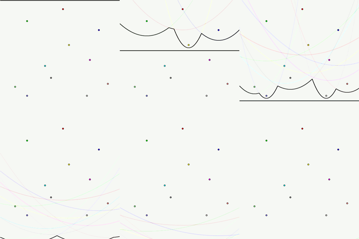
Today, I will give you the outline for Fortune's Sweepline algorithm for determining the Voronoi diagram and Delaunay triangulation of a point set. A picture is worth a thousand words, and so this post will probably clock in at several million as I generate a bunch of animations.


We begin with a point set:


I will then take a horizontal line starting above my point set, and 'sweep' it down across the point set:


I will then do the same thing again, but in addition to the sweep line, I will also take the points above the line, and draw parabolas corresponding to each point as a locus and the sweepline as the directrix:


Now, I will edit the previous animation by only drawing the pieces of the parabolas that are closest to the sweepline. The resulting wavy line is called the beachline, as it resembles the shape of a wave crashing against the beach:


Finally, I will draw the paths taken by the intersection points of adjacent arcs on the beachline:


These intersection points are tracing out the Voronoi edges!


In the next post, we will investigate WHY this process produces the diagram we seek.

Monday, June 29, 2015

Triangulation: Brute Force Delaunay

The story so far: we have a point set we wish to triangulate, and in particular we wish to find the Delaunay triangulation. We also know that Delaunay traingulations are dual to Voronoi diagrams, and so in theory we can solve either problem to come up with the answer to the other. How can we get a computer do to this for us?

Of the two, I consider the Delaunay triangulation to be the more natural representation for a computer. The reason is that Voronoi diagrams, due to the distant Voronoi vertex property, could be arbitrarily large in size, which poses problems for finite-precision computers. Delaunay triangulations, in contrast, are always bounded by the convex hull of the input point set. In addition, the Delaunay edges always have both ends at finite vertices, while Voronoi diagrams have at least three edges that radiate out towards a point at infinity. Therefore, let us make a computer compute a Delaunay triangulation for us.

There is a trivial brute-force algorithm for Delaunay triangulation:

  1. Generate a list of all potential triangles by taking triples of points from the point set. There are at most (N)(N-1)(N-2)/6 distinct triangles.[1]
  2. For each triangle, test whether any other points in the point set are inside its circumcircle. If there are any, throw away the triangle. Otherwise, keep the triangle.

Note: this algorithm does not include special case handling for four or more points lying on a common circle. It will also count any edge not on the convex hull twice.

This algorithm works, but like many brute-force algorithms, it is not good enough. If the input size is N, then there are O(N3) triples of points to consider, and for each triple, we have to compare it to the other N-3 points in the point set. This puts the algorithm's runtime at O(N4), or in layman's terms, "hella slow".[2]

An insightful computer scientist by the name of Fortune was able to find an algorithm to solve this problem in O(N log N) time. In the next post, we will see how he did it. Until then, you could try to solve it yourself.


[1] This is the common 'combination' operator from finite mathematics – N! / [(N-K)! K!] – with K=3.

[2] Binary search is O(log N). Efficient sorting algorithms are O(N log N). Algorithms start to look sluggish once they hit O(N2). Even this slow brute-force algorithm is doing better than O(MN) though, and if you end up with O(N!), you'd better get some coffee, because there's a good chance the universe will end before your algorithm terminates.

Friday, June 26, 2015

Triangulation: Delaunay Triangulations

The story so far: we have looked at the problem of point set triangulation, and had a seemingly-unrelated foray into Voronoi diagrams. How are they related?

The answer is straightforward. Start with a point set:

Then, create from it a Voronoi diagram:

Then, add an edge between two points if their corresponding Voronoi cells meet along a Voronoi edge:

Voila. A triangulation of the point set. Specifically, it is a Delaunay triangulation of the point set, named after some mathematician (not) named Delaunay. Delaunay triangulations have the useful property that they avoid skinny triangles, which I previously mentioned are things you want to avoid when you are sending the triangles to a 3D rendering pipeline.

Every point set has a unique Voronoi diagram. It so happens that most point sets also have a unique Delanuay triangulation. For those that do not, the reason why is straightforward to detect: it happens when four or more of the points in the point set are cocircular, and no other points are within that circle. You can also see this when the Voronoi diagram has four or more sites meeting at a common Voronoi vertex (in the general case, Voronoi vertices only have degree 3). When such a cocircular point grouping is found, the Voronoi diagram cannot be used to triangulate the polygon containing those points. Fortunately, they are easy to triangulate: they are convex polygons (all polygons made from vertices lying on a circle, 'circumscribed polygons', are convex), and you can triangulate a convex polygon by picking a vertex at random and connecting it to every other vertex in the polygon.

It so happens that Delaunay triangulations and Voronoi diagrams are dual graphs of one another. This fact is apparent from how we constructed the Delaunay triangulation from the Voronoi diagram, but you can also construct a Voronoi diagram from a Delaunay triangulation. In this case, you create a Voronoi vertex for each triangle in the triangulation, and locate that vertex at the circumcenter of the triangle's points. Then, you connect Voronoi vertices by line segments which bisect the edges of the triangulation. Here again, if you have circumscribed polygons in the triangulation, you need to do a bit of special case handling, since multiple triangles will have coincident circumcenters.

There is one other oddity worth mentioning in Voronoi diagrams: they can have Voronoi vertices located arbitrarily far away from the points in the point set. If a triangle is obtuse, then its circumcenter lies outside the triangle:

For triangles whose edges are not part of the convex hull of the point set, this is not a problem. However, if you have a point very close to, but not on, the convex hull, then you can get a triangle with an angle arbitrarily close to 180 degrees, which pushes its circumcenter close to the point at infinity. (Estimates say that the circumcenter can get almost 2/3 of the way to the point at infinity)[1].

This 'distant Voronoi vertex' property is not really a problem in practice, although it is important to keep in mind if you are using a Voronoi diagram to produce a Delaunay triangulation. If you have a finite sheet of paper, then you might have Voronoi cells that touch, but only at locations outside of your diagram, like the purple cell in the example Voronoi diagram above.

There are two ways to deal with this: check that all of your externally-radiating Voronoi edges are diverging from one another, or just always include the convex hull in your triangulation.

In the next post, we will start looking at how to get a computer to generate a Delaunay triangulation for us.


[1] This is not a valid mathematical statement. Infinity is not a number and so cannot be multiplied by a ratio (other than 0.6[2]).

[2] This is also not a valid mathematical statement.

Wednesday, June 24, 2015

Triangulation: Voronoi Diagrams

In this post, we will look at a practical problem: where should you open a new Blockbuster?

Before we begin, I should point out for younger readers that 'Blockbuster' was the name of a movie rental company that went bankrupt in 2010 and today has more or less ceased to exist (their Wikipedia page says that only private franchises still operate). I should also point out that 'movie rentals' were things that people did to watch movies before the existence of Netflix. For the purposes of this post, we will assume it is 2003, when Blockbuster was making a lot of money and doing well as a company, so they were actually opening new stores instead of shutting down old ones.

You have been asked to select the site of a new Blockbuster store in an existing city with several stores already open. In the real world, there are a lot of different factors that influence this decision: population density, property costs, transportation accessibility and competitors being just four I could come up with off the top of my head. For this post, we will consider only the three tenets of real estate: location, location, and location.

All else being equal, a Blockbuster customer will go to the closest store to their home. They will also not go to Blockbuster at all if the closest store is still further away then their Laziness Quotient. (Incidentally, a large part of the reason that Netflix destroyed Blockbuster was that it reduced the Laziness Quotient of nearly everyone to essentially zero.) This suggests that our new store should be selected to be as far away as possible from other stores. This will maximize new customers, and minimize duplicate coverage, which does not give you any new business. (As an extreme example, if your new location was across the street from an existing store, you would succeed in getting zero new customers, and have two stores that were only doing half as much business as the old one did.)

To solve this problem, you begin by taking a map of your store locations, and assigning each location a colour:

You then colour the rest of the map according to the following rule: the colour at a given point should be the same colour as the closest store:

The resulting image is known as a Voronoi diagram, after some mathematician named Voronoi. It can be used as the basis of a solution for the 'nearest neighbour' problem: given a point, which of a set of points is closest? If you were to pin a Voronoi diagram to a wall and throw a dart at it, the colour it hits would correspond to the nearest neighbour answer. Each region of colour shall be called the Voronoi cell for a given point, called a Voronoi site.

It is not difficult to prove that at the border between two cells, called a Voronoi edge, the distance between that border and the two sites is equal. It is also not difficult to prove that at the points where three or more cells meet, called a Voronoi vertex, the distance between that point and the cell's sites are all equal. Astute readers will immediately note that this sounds an awful lot like the circumcircle of the points.

The answer to the problem, therefore, is to pick the Voronoi vertex with the largest circumcircle of the original points, and open the new Blockbuster at that point.

Readers of the blog will note an uncharacteristic finality in that answer. Surely, I am going to go on to other special cases, or places where that approach does not work? I am not. I have already noted that this approach ignores a whole host of other urban planning factors, but in terms solely of location, it is the best choice.

I will, however, go on to note that Voronoi diagrams have a whole host of uses. One of the most interesting ones to me was its use in one of the founding experiments of epidemiology. In 1854, there was a serious cholera epidemic in London. Back then, the cause of cholera (a bacterial infection) was not known. A physician by the name of John Snow, usurping George R. R. Martin by over a century, was trying to determine a cause, or cure, or treatment to the epidemic. His great insight led him to take a map of London, and to overlay a Voronoi diagram generated by using the locations of water pumps as the sites. He then plotted the homes of all of the infected and deceased victims of the epidemic. Nearly all of the infected were within a single Voronoi cell: that of the Broad Street water pump. The evidence that this pump was responsible was strong enough that the city council had the water pump's handle removed to prevent further transmission of the disease.

As mentioned above, Voronoi diagrams can be used to efficiently compute nearest-neighbour operations, which are common in geometric algorithms. They can also be used as a texture-generating primitive, in similar fashion to the more well-known Perlin noise, which is the video game development application of choice for this blog.

Finally, the diagrams make for pretty pictures. The joke in 'A Brief History of Time' is that each formula would halve the readership of Stephen Hawking's novel; my hope is that each Voronoi diagram I add to my posts will double its readership.

In the next post, I will reveal the terrible secret connecting Voronoi diagrams to point set triangulation.

Monday, June 22, 2015

Triangulation: Introduction

In this post, we will move away from the abstract mathematics of the last several posts, and onto a very practical problem: point set triangulation.

Point set triangulation, like every interesting problem in computer science, is actually quite straightforward at first glance. The problem starts with a set of distinct points on a two-dimensional plane, like so:

One note before we continue: there is a restriction on the points, and that is that they are not all colinear. If they all lie on a single, common line, you would not be able to draw a triangle between three of the points. For the rest of this article, we will assume that the input point set is not degenerate. We will also assume that the input point set contains at least three points: otherwise, you couldn't draw a triangle at all!.

A solution to the problem is a set of straight edges connecting the points in the point set, with the following requirements:

  • The edges of the convex hull of the point set must be included
  • The graph must be connected (ie, there must be a path between every pair of points) and planar (ie, lines cannot cross, but may meet at one of the points)
  • Every face (except the outer face) must be a triangle (hence, you are 'triangulating' the points)

Here is a solution for the point set above:

As I said, this is straightforward at first glance. If I drew a bunch of dots on a piece of paper, and gave you a pencil and a ruler, I have no doubt that you could solve the problem with no mathematical or programming training. (Give it a try!)

I can assure you, however, that the problem is richer if you give it a second glance. For instance, if I gave the same set of points to two different people, it is quite likely that I would get back two different solutions:

Which solution is correct? They both are. In general, point sets do not have unique triangulations, although there are exceptional cases that do.[1]

Before we examine the problem more closely, we should first answer that most pivotal of philosophical questions, "who cares?" Specifically, why would anyone want to triangulate a point set? Like almost everything on this blog, we find an application in video game development: height maps. Here, we have a regular grid of X,Y sample points (although regularity is not required), and each sample point has an associated height value Z. If we triangulate the points based off of their X,Y coordinates, and then draw triangles corresponding to the full X,Y,Z triple, we get a 3D model of terrain suitable for the ground of, say, an outdoor 3D game. As an example, the ground of World of Warcraft is a height map.

We will now transition from the realm of theory to that of practice. In theory, any triangulation of the point set is as good as any other: each meets the criterion specified. In applications, however, we sometimes find that one triangulation is 'better' than another. For instance, consider the following two triangulations of the same point set:

Now, consider if those points were assigned a Z value equal to their distance from the center of the diagram. In the first triangulation, the resulting terrain mesh would be a crater-shaped depression. In the second triangulation, the same points would have produced a pair of depressions more closely resembling a wall socket. Which solution is correct in this case? It depends on your application, but I believe that most people would consider the first triangulation to more correctly match the terrain if we are considering height maps.

There are numerous strategies for selecting a 'best' triangulation for an application. Maybe you want to make sure that your triangles do not have small angles; this is the case in 3D engines, where 'skinny' triangles tend to lead to numerical instability during rendering. Maybe you want to minimize the sum of the lengths of the edges; this is the case if your points represent cities on a map and you want to build roads between them. Maybe you just want to compute the triangulation quickly and are willing to trade speed for optimality and settle for an answer that only approximately meets your other criteria.

There are two things you can't come up with strategies for, however: the number of triangles or the number of edges. Every triangulation of a given point set has the same number of triangles and edges; these are both specified as a function of the number of vertices and the number of vertices which are part of the convex hull of the point set. Specifically, you will have 2(v - 1) - h triangles, and 3(v - 1) - h edges. (A handy mnemonic for remembering these formulas is to note the formulas are the same except for the constant 2 or 3, and that E and 3 are similar in shape.)

In the next post, we will look at a seemingly unrelated geometry problem which will turn out to have a very useful side effect for the problem of point set triangulation.


[1] One configuration of points that admits a unique triangulation is N points, where N-1 of those points are collinear. The resulting triangulation will have a fan shape, where every collinear point is connected to the 'outlier' point:

As a special case, note that if you have N = 3 points, you always satisfy this criterion: pick any two points, and they give you a line, and the third point won't be on that line. Thus, the triangulation of three points is unique. (It is exactly the triangle formed with those three points as vertices.)

It is important to note, however, that as soon as you have a second 'outlier', the uniqueness of the solution is lost, as can be seen with the 'crater height map' example, above.

There may be other configurations; but off hand I do not know them, and I suspect they do not exist.

Friday, May 15, 2015

Sorting Circles 3: Implementation

To finish off the last two posts, here is an implementation of the circle sorting algorithm as a Python script. The method, order_circles, accepts as input the x, y and quadrance of two circles, and returns -1 if C1 < C2, or returns 0 if C1 = C2, or returns 1 if C1 > C2. The ordering is based on descending order of the circle bottoms, but the x-coordinate is used as a tiebreaker.

This design is slightly different than a native speaker of Python might design it: they would typically implement the algorithm as a true/false result depending on whether C1 < C2. I implemented the three-return-code result for two reasons: I am a native C# speaker, where the IComparable interface rules, and because I found the Python way to be a bit less elegant when I was implementing the tiebreaker code. It's trivially easy to convert my answer to the Python one, if you are so inclined.

CIRCLE_1_FIRST = -1
CIRCLES_EQUAL = 0
CIRCLE_2_FIRST = 1

def order_circles(x1, y1, q1, x2, y2, q2):
 result = order_circle_bottoms(y1, q1, y2, q2)
 
 if result == CIRCLES_EQUAL:
  result = order_numbers(x1, x2)

 return result


def order_circle_bottoms(y1, q1, y2, q2):
 if q1 == q2:
  return order_numbers(y2, y1)
  
 if q1 < q2:
  yS,qS = y1,q1
  yL,qL = y2,q2
  invert = 1
 else:
  yS,qS = y2,q2
  yL,qL = y1,q1
  invert = -1
  
 if yS >= yL:
  return CIRCLE_1_FIRST * invert
 elif pow(yL - yS, 2) > qL:
  return CIRCLE_2_FIRST * invert
 else:
  yC = (pow(yS, 2) - pow(yL, 2) + qL - qS) / (2 * (yS - yL))
  return order_numbers(qS, pow(yC - yS, 2)) * invert


def order_numbers(a, b):
 if a < b:
  return CIRCLE_1_FIRST
 elif a > b:
  return CIRCLE_2_FIRST
 else:
  return CIRCLES_EQUAL

#------------------------------------------------------------------------------------

def test_case(desc, x1, y1, q1, x2, y2, q2, expected):
 if (order_circles(x1, y1, q1, x2, y2, q2) == expected and
  order_circles(x2, y2, q2, x1, y1, q1) == -expected):
  print('PASS\t' + desc)
 else:
  print('!FAIL!\t' + desc)
 
test_case('Equal circles', 0, 0, 4, 0, 0, 4, CIRCLES_EQUAL)
test_case('Same size circles', 0, 1, 4, 0, 0, 4, CIRCLE_1_FIRST)
test_case('Same center circles', 0, 0, 1, 0, 0, 4, CIRCLE_1_FIRST)
test_case('Smaller circle higher', 0, 10, 1, 0, 0, 4, CIRCLE_1_FIRST)
test_case('Smaller circle beneath larger', 0, 0, 4, 0, -10, 1, CIRCLE_1_FIRST)
test_case('Smaller circle inside larger', 0, 0, 1, 0, 5, 100, CIRCLE_1_FIRST)
test_case('Smaller circle poking out of larger', 0, 3, 16, 0, 0, 4, CIRCLE_1_FIRST)
test_case('Unequal circles tangent', 0, 1, 1, 0, 2, 4, CIRCLES_EQUAL)
test_case('Equal circles x order', 0, 0, 4, 1, 0, 4, CIRCLE_1_FIRST)
test_case('Unequal circles tangent x order', 0, 1, 1, 1, 2, 4, CIRCLE_1_FIRST)

Wednesday, May 13, 2015

Sorting Circles 2: The Answer

First, we formally state the problem: we are looking for a partial order of a set of circles Cn, defined by a point (Xn, Yn) and a quadrance Qn, according to the following relation:

C1 ≤ C2 ⇔ Y2 - sqrt(Q2) ≤ Y1 - sqrt(Q1)

Note carefully that the coeffiecients one one side of the relation are flipped from the other side; this is because the circles are ordered top-to-bottom, so the 'least' circle will be the highest one. Note also that Xn does not appear anywhere in this relation, so without loss of generality, we may assume that Xn = 0. Informally, translation the circles horizontally doesn't affect their order. In practice, we can use the X values of the circle centers as a tiebreaker if the first relation says that the circles would be equal.

Our problem is made more complicated by the fact that we cannot always take the square root of a quadrance, so we seek an algorithm that will give the correct answer without having to leave the domain of natural numbers. We can start with a special case of the two circles being the same size; that is, Q1 = Q2. In this case, although we can't take the square root of either, we know that the square root of both is the same, and so we can just subtract whatever its value would be from both sides of the inequality:

C1 ≤ C2 ⇔ Y2 ≤ Y1

Informally, this case shows that for two circles the same size, then the higher one comes first in the ordering, as in this example:

We can cross off another special case if the two circles are centered at the same height; that is, Y1 = Y2:

C1 ≤ C2 ⇔ -sqrt(Q2) ≤ -sqrt(Q1)
C1 ≤ C2 ⇔ sqrt(Q1) ≤ sqrt(Q2)
C1 ≤ C2 ⇔ Q1 ≤ Q2

The last step in this derivation comes from the fact that the square root function is monotonic; that is, x ≤ y ⇔ f(x) ≤ f(y). We can't actually determine the value of the square root, but we don't need the actual value to know which one is greater. Informally, this case shows that for two circles centered at the same height, the smaller one comes first in the ordering, as in this example:

At this point we have exhausted any equivalences between the two circles, so Q1 ≠ Q2 and Y1 ≠ Y2 for the remainder of this discussion. Let's see if we can make any more progress by rearranging the relation:

C1 ≤ C2 ⇔ Y2 - sqrt(Q2) ≤ Y1 - sqrt(Q1)
C1 ≤ C2 ⇔ Y2 + sqrt(Q1) - sqrt(Q2) ≤ Y1
C1 ≤ C2 ⇔ sqrt(Q1) - sqrt(Q2) ≤ Y1 - Y2

Let us make a few assumptions and see where they lead:

Q1 < Q2
sqrt(Q1) < sqrt(Q2)
sqrt(Q1) - sqrt(Q2) < 0
Y2 < Y1

0 < Y1 - Y2

sqrt(Q1) - sqrt(Q2) < Y1 - Y2
C1 < C2

An equivalent derivation will show that Q2 < Q1 and Y1 < Y2 implies that C2 < C1. Informally, this case shows that if the circle with the higher y-coordinate is also smaller, then it comes first in the ordering, as in this example:

We seem to be narrowing in on the answer. At this point, we know that the only unconsidered case is the one where the larger circle has the higher center. That is, QL > QS and YL > YS. In actuality, we are still where we started, because even under these constraints, the relative ordering of the two circles could still be any of the three possible answers.

We can knock out one final special case. Make the following assumption, and see where it leads:

QL < (YL - YS)2
sqrt(QL) < YL - YS
YS < YL - sqrt(QL)
YS - sqrt(QS) < YL - sqrt(QL)
⇔ CL < CS

Informally, we know already that the smaller circle is below the larger one. If the smaller circle is also outside of the larger one (because the squared distance between the two circle centers is larger than the quadrance of the larger circle), then the smaller circle must come second in the order, since its bottom must be lower than that of the larger circle, as in this example:

We are still where we started, though. The smaller circle is centered lower than the larger circle, and is inside it. It may be poking outside of the larger circle though, in which case it should come second in the ordering. It may be fully within the larger circle, in which case it should come first in the ordering. Or it may be the case that the two circles are just touching at their bottoms, in which case the two circles are 'equal' under the ordering. How can we tell?

The answer is to count the number of intersection points between the two circles, after the circles have been translated to have their centres on the Y axis (ie, X = 0). If there are no intersection points, then we have the 'smaller circle inside larger one' case and the smaller circle comes first. If there is one intersection point, then we have the 'circles touching at the bottom' case and they are equal. If there are two intersection points, then we have the 'smaller circle poking out of the larger one' case, and the larger circle comes first.

It is important to note, however, that in order for this answer to be correct, the special cases already proven above have to be ruled out. If the two circles centered on the Y axis meet at exactly one point, then in the general case, the top or bottom of the smaller circle might be touching the top or bottom of the larger circle, for a total of four possibilities. The fact that the smaller circle is centered below the larger one rules out that they are touching at the larger circle's top, and the fact that the smaller circle's center is inside the larger circle rules out that the smaller circle's top is touching the larger circle's bottom.

To find the circle's intersections, we start by observing that the intersections, if any, lie on both circles. The larger circle's points satisfy the equation x2 + (y - YL)2 = QL, and similarly, the smaller circle's points satisfy the equation x2 + (y - YS)2 = QS. Therefore, we have:

x2 + (y - YL)2 - QL = 0 = x2 + (y - YS)2 - QS
(y - YL)2 - QL = (y - YS)2 - QS
y2 - 2YLy + YL2 - QL = y2 - 2YSy + YS2 - QS
2(YS - YL)y = YS2 - YL2 + QL - QS
y = [YS2 - YL2 + QL - QS] / 2(YS - YL)

Call this quantity yI; I for intersection. The x-coordinates of the intersection point(s) can be found by subbing this back into one of the circle equations:

x2 + (y - YS)2 = QS
x2 + (YI - YS)2 - QS = 0

Here we have a quadratic equation with a = 1, b = 0, and c = (YI - YS)2 - QS. Its determinant, b2 - 4ac, is simply -4c. We thus know the following:

  • CS < CL ⇔ zero intersections between circles ⇔ -4c < 0 ⇔ 0 < c ⇔ 0 < (YI - YS)2 - QS ⇔ QS < (YI - YS)2
  • CS = CL ⇔ one intersections between circles ⇔ -4c = 0 ⇔ 0 = c ⇔ 0 = (YI - YS)2 - QS ⇔ QS = (YI - YS)2
  • CS > CL ⇔ two intersections between circles ⇔ -4c > 0 ⇔ 0 > c ⇔ 0 > (YI - YS)2 - QS ⇔ QS > (YI - YS)2

The salient facts being:

  • CS < CL ⇔ QS < (YI - YS)2
  • CS = CL ⇔ QS = (YI - YS)2
  • CS > CL ⇔ QS > (YI - YS)2

Informatlly, this test is comparing the squared distance between the intersection line and the circle center to the circle's quadrance (the squared distance between the circle's edge and the circle center).


That was a long one, so let's wrap it up with a handy chart:

Q1 < Q2 Q1 = Q2 Q1 > Q2
Y1 < Y2 special C1 > C2 C1 > C2
Y1 = Y2 C1 < C2 C1 = C2 C1 > C2
Y1 > Y2 C1 < C2 C1 < C2 special

In the special case, the smaller circle's center is lower than the larger circle. If the smaller circle's center is completely outside the larger circle, then the larger circle is the 'lesser' circle. Otherwise, the order of the two circles is determined by the number of points at which the circles intersect: zero for smaller circle first, one for circles equal, or two for larger circle first.

Monday, May 11, 2015

Sorting Circles

In today's post, we are going to consider a simple problem, and do it the hard way.

The problem is this: We are given a set of circles in the 2D plane. These circles are defined by the X and Y coordinates of their center, and by the square of their radius, Q = r2. All three of these values are rational numbers. We are then tasked to sort the circles according to the following order: circle 1 comes before circle 2 if the bottom of circle 1 is above the bottom of circle 2. As an example, the following circles are in the order we want:

The easy way to do this problem is straightforward. The bottom of each circle is the point (X, Y - sqrt(Q)), a point that is not necessarily rational. Fortunately, the irrational numbers are well-ordered, so we can still sort the circles by this bottom point, from largest to smallest Y-coordinate

As I mentioned at the start, however, we are not going to solve this problem the easy way. We wish to remain in the domain of rational numbers, and so we will ban the use of the square root function when considering our solution.

I am sure this decision will raise a few questions, which I will attempt to address:

Why are all three values rational? Behind the scenes, these circles are defined as the circle containing three distinct points, as discussed in a previous post. Each of these three points are specified in rational coordinates, and the equation derived for their circumcircle shows that the center of the circle is also a rational point. Additionally, the square of the distance between two points is also a rational number. The actual distance may not be rational, however. If you want a counterexample, take the three points (-1, 1), (1, 1), and (1, -1), which are all a distance of sqrt(2) from the origin.

Why is the squared radius denoted Q? Q stands for quadrance, a concept I borrowed from an interesting looking Wikipedia page about 'rational trigonometry'.

What do you have against irrational numbers? Theoretically, nothing. Practically, they are anathema to a computer, which can only truly work with integers. Floating-point numbers are a conceit that trades accuracy for range, and if you aren't careful, you will get the wrong answer due to accumulated round-off errors, and all of your numerical tests are studded with epsilons that turn y = c into |y - c| ≤ 1.0-6 for some arbitrarily-chosen exponent. If you use a solid rational number library, your answers will be guaranteed to be correct with knife-edge precision.

Your proposed rational number library will be slower. First, that's not a question. Second, will it? Probably, but I will practically guarantee that you've made this statement as a knee-jerk reaction; more than half of all statement of 'x is slower' being used to justify a particulary technical approach are based on no actual data. Third, who cares? If it's twice as slow, and the slower algorithm still finishes in 10ms, then doubling its speed isn't going to make your user any happier. We're not writing a real-time operating system today. Correctly getting the right answer is our aim, not quickly getting a wrong answer.

Exactly why are you sorting circles this way? The reason why will have to wait for a future post. For now, let it be sufficient that this is a problem of mathematics, and the search for an answer is of value, not an application of the answer.

What is the answer? Give it some thought. I'll tell you in the next post.